Data Manipulation - reshape2 and plyr

Prepared by Umihiko Hoshijima, Inspiration/Material from Sean Anderson in Reshape2 and plyr

Reshaping data in R

Download data files here

Get the exercise answers

As scientists, we format datasheets to make our data entry intuitive. However, different forms of data analysis in R can require data in different formats. Manipulating data for various analyses and visualization can be facilitated by the package reshape2.

For our example, we will look at our dataset iris, which is a famous statistics dataset that measures the length and width of both sepals and petals on three species of irises (50 individuals each, 150 flowers total). You used iris for your previous ggplot lesson.

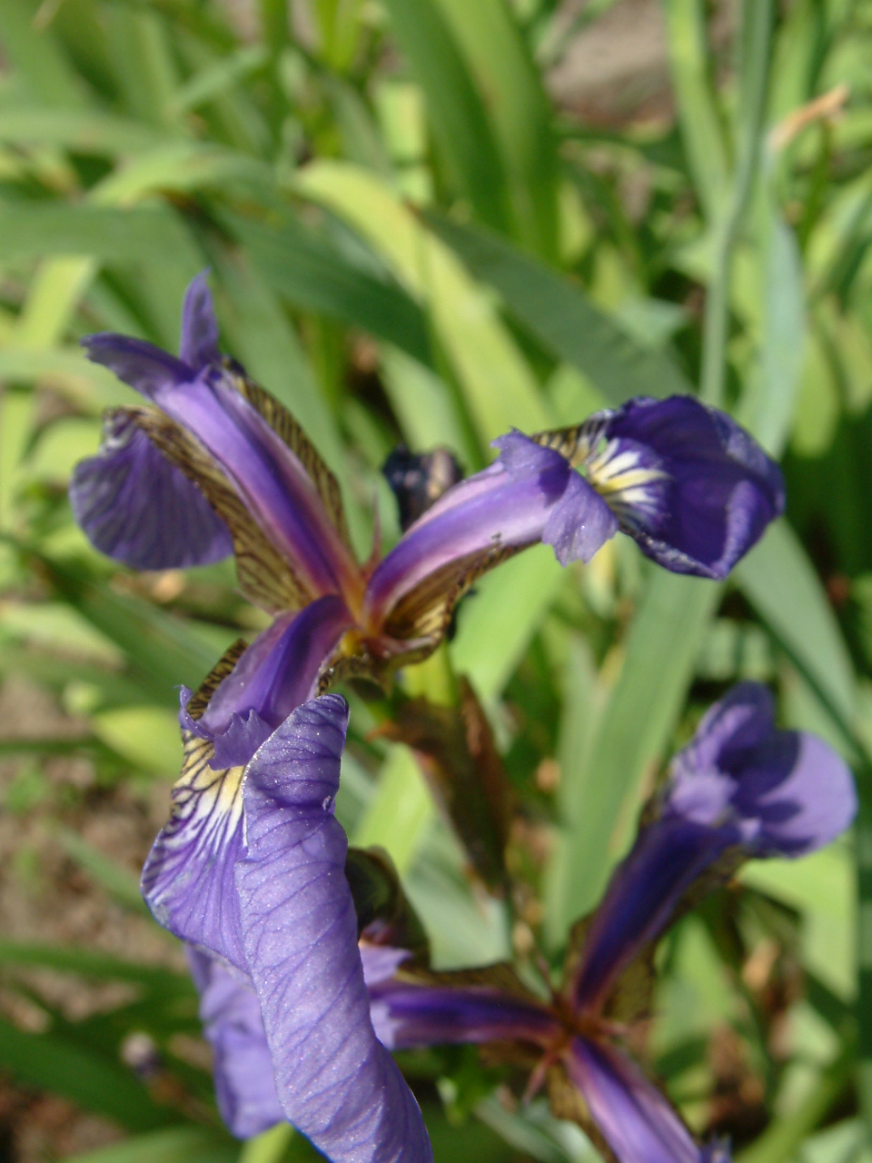
Iris setosa, one of the species you will be looking at. Wikipedia Commmons

This data seems perfectly formatted for many of the plots you conducted. Each individual has a single row, with columns corresponding to the individual measurements as well as the species. Now let's now do a boxplot, comparing the distribution of Sepal.Length between each species:

ggplot(iris, aes(x = Species, y = Sepal.Width)) + geom_boxplot()

Suppose we want to make four boxplots, to compare between species for each flower measurement. In the last lesson we used facet_grid() to divide our data based on the values contained in a certain column. Knowing this, it sounds as though you need a column that says Sepal.Width, Sepal,Length, Petal.Length, Petal.Width… but we don't really have that here. In order to subdivide our measurements and plot each dimension on a different plot, we will need to reformat the dataset so there is only one measurement on each row.

Essentially we want to go from this:

Sepal.Length	Sepal.Width	Petal.Length	Pedal.Width	Species	Individual
5.1	3.5	1.4	0.2	setosa	1
4.9	3.0	1.4	0.2	setosa	2
4.7	3.2	1.3	0.2	setosa	3

To this:

Species	Individual	Measurement	Value
setosa	1	Sepal.Length	5.1
setosa	1	Sepal.Width	3.5
setosa	1	Petal.Length	1.4
setosa	1	Petal.Width	0.2
setosa	2	Sepal.Length	4.9
setosa	2	Sepal.Width	3.0
setosa	2	Petal.Length	1.4
setosa	2	Petal.Width	0.2
setosa	3	Sepal.Length	4.7
setosa	3	Sepal.Width	3.2
setosa	3	Petal.Length	1.3
setosa	3	Petal.Width	0.2

Luckily for us, there's a package in R called reshape2 that can help you manipulate datasets like this. This package has two key functions: melt and dcast. For what we want to do (get rid of columns, add rows), we would use melt. For the opposite, use dcast. Think of it like working with metal - you can melt metal to elongate it vertically, and you can cast it to go back.

To add the individual column into our result, let's first make that column in our iris dataframe. the function dim gives us a list with 2 values: the rows and columns in the dataframe. We only want the number of rows, so we're going to go with:'

nRows <- nrow(iris)
iris$Individual <- 1:nRows
head(iris)

Now we can melt()! Let's see what happens when we call the function:

install.packages('reshape2')
library(reshape2)
iris2 <- melt(iris)
View(iris2)

Huh, that didn't do exactly what we wanted it to do. By default, melt will get rid of all columns with numerical values. Since we want to hold on to the Individual row, we have to manually tell melt what columns we want to keep.

iris2 <- melt(iris, id.vars =  c("Individual", "Species"))

Now let's plot our boxplot. We don't really need facet_grid(), which lets you designate two different variables to divide up the dataset by. We just want it divided by variable, as shown below.

ggplot(iris2, aes(x = Species, y = value))+geom_boxplot()+facet_wrap(~variable)

Unlike facet_grid, which will display all of your plots horizontally or vertically with just one categorizing variable, facet_wrap will wrap them into a grid and keep them nice and tidy. You can even specify the number of rows and columns:

ggplot(iris2, aes(x = Species, y = value))+geom_boxplot()+facet_wrap(~variable, ncol = 3)

As an exercise, let's put our data back to its original shape usingdcast. This has a slightly different syntax, and is in the shape of a formula. We put our id variables (the same ones we specified in melt) on the left of the ~, and put the variable on the right.

iris3 = dcast(iris2, Individual+Species ~ variable)

This forumla can be a bit unintuitive at first, so don't feel discouraged if you don't get it the first time!

EXERCISE 1 - Reshaping Aneurysm.

open up aneurysm_data_site-1.csv. In four individual subplots divided by aneurysm condition (Aneurisms_q1, q2, q3, q4), Plot the Blood Pressure against the respective aneurysm condition. Color the scatterplot based on the age of the patient. When you are done, retrace your steps using dcast() to reshape your melted dataframe back into its original shape.

Summarizing and Operating: the dPlyr world

For our next section, let's load the file mammal_stats.csv from the data folder. This is a subset of a "species-level database of extant and recently extinct mammals.

So far we've successfully loaded data by navigating to the directory and typing the name into read.csv(). But what if we're writing the script for another computer, or for a collaborator that may have the data in a different location? We can instead have the script pop up a window to select their data from.

# Instead of this: 
# mammals <- read.csv("mammal_stats.csv")
# Use this: 
mammals <- read.csv(filename = file.choose())
#mammals.directory=dirname(filename)
#mammals.filename=basename(filename)

The function file.choose() is what pulls up the window and lets you select a file. It then returns that file name and directory, which gets used by read.csv(). The next two rows are optional, but let you extract the directory and the file name of the csv that you pulled from. You can use this when outputting your results by naming them based on the input (Example: input file name is "data1.csv", output file name is "data1_processed.csv").

Alright, back to mammals! You'll notice that as we work on larger datasets, viewing and visualizing the entire dataset can become more and more difficult. Similarly, analyzing the datasets becomes more complex. Is there a good way to be able to summarize datasets succinctly, and to be able to analyze subsets of a dataset automatically?

The answer lies in a handy library called dplyr. dplyr will allow us to perform more complex operations on datasets in intuitive ways.

First off, though, let's explore some very handy sorting and viewing functions in dplyr. glimpse() is a quick and pretty alternative to head():

install.packages('dplyr')
library(dplyr)  
head(mammals)
glimpse(mammals)

Tip: You may see people using require() in their code instead of library(). This is not advised in most cases, as it can make it difficult to trace mistakes in your code.

If i want to shrink the dataset, we can select() columns. We can do that either manually (by naming the columns we want), or by using an operation. where the column name contains() a certain string, or starts_with() or ends_with() one.

select(mammals, order, species) #narrows down to these two columns
select(mammals, species, starts_with("adult")) #the column species, and any column that starts with "adult"
select(mammals, -order) #every row, except `Order`.

We can also select certain rows using the function filter(). As rows aren't named the same way columns are, we will instead use the logical operators >, < , ==, etc. to select the rows we want.

filter(mammals, order == "Carnivora") # only carnivores
filter(mammals, order == "Carnivora" & adult_body_mass_g < 5000) # only carnivores smaller than 5kg
filter(mammals, order == "Carnivora" | order == "Primates") #Any carnivore or primate

We can also arrange the rows in a dataset based on whichever column you want, using arrange().

head(arrange(mammals, adult_body_mass_g)) #row 1 is the smallest mammals, the bumblebee bat. 
head(arrange(mammals, desc(adult_body_mass_g))) #sorts by descending. row 1 is the blue whale. 
head(arrange(mammals, order, adult_body_mass_g)) #sorts first alphabetically by order, then by mass within order. 

EXERCISE 2 - irises

Go back to your iris data. How many setosa have a Sepal.Length greater than 5? Which species has the flower with the longest petal length? The shortest?

The bumblebee bat. Wikipedia Commmons

With these large datasets, dplyr lets you quickly summarize the data. It operates on a principle called split - apply - recombine : we will split up the data, apply some sort of operation, and combine the results to display them. Suppose we want to find the average body masss of each order. We first want to split up the data by order using the function group_by(), apply the mean() function to the column adult_body_mass_g, and report all of the results using the function summarise().

a <- group_by(mammals, order)
summarize(a, mean_mass = mean(adult_body_mass_g, na.rm = TRUE))

To we can add other functions here, such as max(), min(), and sd().

summarize(a, mean_mass <- mean(adult_body_mass_g, na.rm = TRUE), sd_mass <- sd(adult_body_mass_g, na.rm = TRUE))

Tip: inside of these inner parenthesees you MUST use equals signs instead of arrows. Read more here.

summarize makes a new dataset, but mutate will add these columns instead to the original dataframe.

a <- group_by(mammals, order)
mutate(a, mean_mass <- mean(adult_body_mass_g, na.rm = TRUE))

This outputs the same numbers as the equivalent summarize function, but puts them in a new column on the same dataset.

What if we want to figure out how the mass of each animal relates to other animals of its order? To do this, we will divide each species' body mass by its order's mean body mass.

a <- group_by(mammals, order)
mutate(a, mean_mass <- mean(adult_body_mass_g, na.rm = TRUE), normalized_mass <- adult_body_mass_g / mean_mass)

You might be noticing that in each of these examples, we are feeding the result of the first line into the second line, using a as an intermediate variable. While this is functional, there is a more legible solution called Pipes. Pipes uses the operation %>% to push the results of one line to the next. for example, instead of writing

a = group_by(mammals, order)

we would write

install.packages('magrittr')
library(magrittr)

a = mammals %>% #take the mammals data
    group_by(order) %>% #split it up by "order"

The package is named after René Magritte, a surrealist painter who painted "The Treachery of Images" above. This painting is currently on display at the LA County Museum of Art! Wikipedia Commmons

This can make it easy to follow the logical workflow, which makes more and more sense as your operations become more complex. Suppose we want to find the organisms with the biggest mass relative to the rest of its order. We want to split the data by order, apply the mutate functions from above, sort by normalized_mass, and only display the species, adult_body_mass_g, and normalized_mass columns. In longhand it would look like this:

a = group_by(mammals, order)
b = mutate(a, mean_mass = mean(adult_body_mass_g, na.rm = TRUE), normalized_mass = adult_body_mass_g / mean_mass)
c = arrange(b, desc(normalized_mass))
d = select(c, species, normalized_mass)

pipes makes it less messy by reducing the number of variables:

e = mammals %>%
    group_by(order) %>%
    mutate(mean_mass = mean(adult_body_mass_g, na.rm = TRUE), 
    normalized_mass = adult_body_mass_g / mean_mass) %>%
    arrange(desc(normalized_mass)) %>%
    select(species, normalized_mass, adult_body_mass_g) 

This lets us see that many of the animals relatively large for their size are rodents. It seems to make sense that the smaller your order's average mass, the easier it would be to be 116x larger than the average!

EXERCISE 3 - Data exploration. Try to use pipes!

Which species of iris has the longest average sepals? Which species has the smallest variance of sepal length over all of its individuals measured? Which species of carnivore has the largest body length to body mass ratio? (Hint: that's adult_head_body_len_mm / adult_body_mass_g')

Sources and Umi's additional tips/tricks:

• This is where I learned reshape: Sean Anderson as well as dplyr: Sean Anderson. He actually helped me over twitter in suggesting dPlyr - so a shout-out to him for being awesome and accessible!
• This is another dplyr tutorial that may help in addition to that first one: Kevin Markham
• Sometimes dPlyr might not do exactly what you want. In reality, dPlyr is a streamlined version of a more powerful (but slower) library called plyr. Sean Anderson's plyr tutorial. While dplyr always takes in a dataframe and outputs a dataframe (summarize and mutate), plyr can take in a dataframe, list, or array and output a dataframe, list, or array. There are also individual R functions that go from array to array (apply) or data frame to data frame (aggregate) but plyr brings them all under one roof for easier syntax.
• This whole lesson plan is written in Markdown, which lets us have those blocks of code. However, there are ways of making documents where the code actually RUNS. This means you can have code generating figures right inside of your document! The two I would suggest for this are R markdown, which is nice but doesn't give you as much customizability as knitr. knitr (a beefed-up version of another format Sweave) is \LaTeX with blocks of R code embedded. You might use this to give code to your collaborators that you can GUARANTEE works, because the outputs go straight into your document.