Programming with R

Analyzing raptor data

We are studying inflammation in raptors who have been given a new treatment for arthritis, and need to analyze the first dozen data sets. The data sets are stored in comma-separated values (CSV) format. Each row holds the observations for just one raptor. Each column holds the inflammation measured in a day, so we have a set of values in successive days. The first few rows of our first file look like this:

0,0,1,3,1,2,4,7,8,3,3,3,10,5,7,4,7,7,12,18,6,13,11,11,7,7,4,6,8,8,4,4,5,7,3,4,2,3,0,0
0,1,2,1,2,1,3,2,2,6,10,11,5,9,4,4,7,16,8,6,18,4,12,5,12,7,11,5,11,3,3,5,4,4,5,5,1,1,0,1
0,1,1,3,3,2,6,2,5,9,5,7,4,5,4,15,5,11,9,10,19,14,12,17,7,12,11,7,4,2,10,5,4,2,2,3,2,2,1,1
0,0,2,0,4,2,2,1,6,7,10,7,9,13,8,8,15,10,10,7,17,4,4,7,6,15,6,4,9,11,3,5,6,3,3,4,2,3,2,1
0,1,1,3,3,1,3,5,2,4,4,7,6,5,3,10,8,10,6,17,9,14,9,7,13,9,12,6,7,7,9,6,3,2,2,4,2,0,1,1

We want to:

• Load data into memory,
• Calculate the average value of inflammation per day across all raptors, and
• Plot the results.

To do all that, we’ll have to learn a little bit about programming.

Loading Data

To load our inflammation data, first we need to tell our computer where is the file that contains the values. We have been told its name is inflammation-01.csv. This is very important in R, if we forget this step we’ll get an error message when trying to read the file. We can change the current working directory using the function setwd. For this example, we change the path to the directory we just created:

setwd("~/Desktop/software-carpentry-2016/data-files/r-lesson/")

Just like in the Unix Shell, we type the command and then press Enter (or return). Alternatively you can change the working directory using the RStudio GUI using the menu option Session -> Set Working Directory -> Choose Directory...

The data files are located in the directory data inside the working directory. Now we can load the data into R using read.csv:

read.csv(file = "data/inflammation-01.csv", header = FALSE)

The expression read.csv(...) is a function call that asks R to run the function read.csv.

read.csv has two arguments: the name of the file we want to read, and whether the first line of the file contains names for the columns of data. The filename needs to be a character string (or string for short), so we put it in quotes. Assigning the second argument, header, to be FALSE indicates that the data file does not have column headers. We’ll talk more about the value FALSE, and its converse TRUE, in lesson 04.

The utility of a function is that it will perform its given action on whatever value is passed to the named argument(s). For example, in this case if we provided the name of a different file to the argument file, read.csv would read it instead. We’ll learn more of the details about functions and their arguments in the next lesson.

Since we didn’t tell it to do anything else with the function’s output, the console will display the full contents of the file inflammation-01.csv. Try it out.

read.csv read the file, but we can’t use data unless we assign it to a variable. A variable is just a name for a value, such as x, current_temperature, or subject_id. We can create a new variable simply by assigning a value to it using <-

weight_kg <- 55

Once a variable has a value, we can print it by typing the name of the variable and hitting Enter (or return). In general, R will print to the console any object returned by a function or operation unless we assign it to a variable.

weight_kg

[1] 55

We can do arithmetic with the variable:

# weight in pounds:
2.2 * weight_kg

[1] 121

We can also change an object’s value by assigning it a new value:

weight_kg <- 57.5
# weight in kilograms is now
weight_kg

[1] 57.5

If we imagine the variable as a sticky note with a name written on it, assignment is like putting the sticky note on a particular value:

This means that assigning a value to one object does not change the values of other variables. For example, let’s store the subject’s weight in pounds in a variable:

weight_lb <- 2.2 * weight_kg
# weight in kg...
weight_kg

[1] 57.5

# ...and in pounds
weight_lb

[1] 126.5

and then change weight_kg:

weight_kg <- 100.0
# weight in kg now...
weight_kg

[1] 100

# ...and weight in pounds still
weight_lb

[1] 126.5

Since weight_lb doesn’t “remember” where its value came from, it isn’t automatically updated when weight_kg changes. This is different from the way spreadsheets work.

Now that we know how to assign things to variables, let’s re-run read.csv and save its result:

dat <- read.csv(file = "data/inflammation-01.csv", header = FALSE)

This statement doesn’t produce any output because assignment doesn’t display anything. If we want to check that our data has been loaded, we can print the variable’s value. However, for large data sets it is convenient to use the function head to display only the first few rows of data.

head(dat)

  V1 V2 V3 V4 V5 V6 V7 V8 V9 V10 V11 V12 V13 V14 V15 V16 V17 V18 V19 V20
1  0  0  1  3  1  2  4  7  8   3   3   3  10   5   7   4   7   7  12  18
2  0  1  2  1  2  1  3  2  2   6  10  11   5   9   4   4   7  16   8   6
3  0  1  1  3  3  2  6  2  5   9   5   7   4   5   4  15   5  11   9  10
4  0  0  2  0  4  2  2  1  6   7  10   7   9  13   8   8  15  10  10   7
5  0  1  1  3  3  1  3  5  2   4   4   7   6   5   3  10   8  10   6  17
6  0  0  1  2  2  4  2  1  6   4   7   6   6   9   9  15   4  16  18  12
  V21 V22 V23 V24 V25 V26 V27 V28 V29 V30 V31 V32 V33 V34 V35 V36 V37 V38
1   6  13  11  11   7   7   4   6   8   8   4   4   5   7   3   4   2   3
2  18   4  12   5  12   7  11   5  11   3   3   5   4   4   5   5   1   1
3  19  14  12  17   7  12  11   7   4   2  10   5   4   2   2   3   2   2
4  17   4   4   7   6  15   6   4   9  11   3   5   6   3   3   4   2   3
5   9  14   9   7  13   9  12   6   7   7   9   6   3   2   2   4   2   0
6  12   5  18   9   5   3  10   3  12   7   8   4   7   3   5   4   4   3
  V39 V40
1   0   0
2   0   1
3   1   1
4   2   1
5   1   1
6   2   1

mass <- 47.5
age <- 122
mass <- mass * 2.0
age <- age - 20

Manipulating Data

Now that our data is loaded in memory, we can start doing things with it. First, let’s ask what type of thing dat is:

class(dat)

[1] "data.frame"

The output tells us that is a data frame. Think of this structure as a spreadsheet in MS Excel that many of us are familiar with. Data frames are very useful for storing data and you will find them elsewhere when programming in R. A typical data frame of experimental data contains individual observations in rows and variables in columns.

We can see the shape, or dimensions, of the data frame with the function dim:

dim(dat)

[1] 60 40

This tells us that our data frame, dat, has 60 rows and 40 columns.

If we want to get a single value from the data frame, we can provide an index in square brackets, just as we do in math:

# first value in dat
dat[1, 1]

[1] 0

# middle value in dat
dat[30, 20]

[1] 16

An index like [30, 20] selects a single element of a data frame, but we can select whole sections as well. For example, we can select the first ten days (columns) of values for the first four raptors (rows) like this:

dat[1:4, 1:10]

  V1 V2 V3 V4 V5 V6 V7 V8 V9 V10
1  0  0  1  3  1  2  4  7  8   3
2  0  1  2  1  2  1  3  2  2   6
3  0  1  1  3  3  2  6  2  5   9
4  0  0  2  0  4  2  2  1  6   7

The slice 1:4 means, “Start at index 1 and go to index 4.”

The slice does not need to start at 1, e.g. the line below selects rows 5 through 10:

dat[5:10, 1:10]

   V1 V2 V3 V4 V5 V6 V7 V8 V9 V10
5   0  1  1  3  3  1  3  5  2   4
6   0  0  1  2  2  4  2  1  6   4
7   0  0  2  2  4  2  2  5  5   8
8   0  0  1  2  3  1  2  3  5   3
9   0  0  0  3  1  5  6  5  5   8
10  0  1  1  2  1  3  5  3  5   8

We can use the function c, which stands for combine, to select non-contiguous values:

dat[c(3, 8, 37, 56), c(10, 14, 29)]

   V10 V14 V29
3    9   5   4
8    3   5   6
37   6   9  10
56   7  11   9

We also don’t have to provide a slice for either the rows or the columns. If we don’t include a slice for the rows, R returns all the rows; if we don’t include a slice for the columns, R returns all the columns. If we don’t provide a slice for either rows or columns, e.g. dat[, ], R returns the full data frame.

# All columns from row 5
dat[5, ]

  V1 V2 V3 V4 V5 V6 V7 V8 V9 V10 V11 V12 V13 V14 V15 V16 V17 V18 V19 V20
5  0  1  1  3  3  1  3  5  2   4   4   7   6   5   3  10   8  10   6  17
  V21 V22 V23 V24 V25 V26 V27 V28 V29 V30 V31 V32 V33 V34 V35 V36 V37 V38
5   9  14   9   7  13   9  12   6   7   7   9   6   3   2   2   4   2   0
  V39 V40
5   1   1

# All rows from column 16
dat[, 16]

 [1]  4  4 15  8 10 15 13  9 11  6  3  8 12  3  5 10 11  4 11 13 15  5 14
[24] 13  4  9 13  6  7  6 14  3 15  4 15 11  7 10 15  6  5  6 15 11 15  6
[47] 11 15 14  4 10 15 11  6 13  8  4 13 12  9

Now let’s perform some common mathematical operations to learn about our inflammation data. When analyzing data we often want to look at partial statistics, such as the maximum value per raptor or the average value per day. One way to do this is to select the data we want to create a new temporary data frame, and then perform the calculation on this subset:

# first row, all of the columns
raptor_1 <- dat[1, ]
# max inflammation for raptor 1
max(raptor_1)

[1] 18

We don’t actually need to store the row in a variable of its own. Instead, we can combine the selection and the function call:

# max inflammation for raptor 2
max(dat[2, ])

[1] 18

R also has functions for other common calculations, e.g. finding the minimum, mean, median, and standard deviation of the data:

# minimum inflammation on day 7
min(dat[, 7])

[1] 1

# mean inflammation on day 7
mean(dat[, 7])

[1] 3.8

# median inflammation on day 7
median(dat[, 7])

[1] 4

# standard deviation of inflammation on day 7
sd(dat[, 7])

[1] 1.725187

What if we need the maximum inflammation for all raptors, or the average for each day? As the diagram below shows, we want to perform the operation across a margin of the data frame:

To support this, we can use the apply function.

apply allows us to repeat a function on all of the rows (MARGIN = 1) or columns (MARGIN = 2) of a data frame.

Thus, to obtain the average inflammation of each raptor we will need to calculate the mean of all of the rows (MARGIN = 1) of the data frame.

avg_raptor_inflammation <- apply(dat, 1, mean)

And to obtain the average inflammation of each day we will need to calculate the mean of all of the columns (MARGIN = 2) of the data frame.

avg_day_inflammation <- apply(dat, 2, mean)

Since the second argument to apply is MARGIN, the above command is equivalent to apply(dat, MARGIN = 2, mean). We’ll learn why this is so in the next lesson.

animal <- c("m", "o", "n", "k", "e", "y")
# first three characters
animal[1:3]

[1] "m" "o" "n"

# last three characters
animal[4:6]

[1] "k" "e" "y"

Plotting

The mathematician Richard Hamming once said, “The purpose of computing is insight, not numbers,” and the best way to develop insight is often to visualize data. Visualization deserves an entire lecture (or course) of its own, but we can explore a few of R’s plotting features.

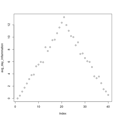
Let’s take a look at the average inflammation over time. Recall that we already calculated these values above using apply(dat, 2, mean) and saved them in the variable avg_day_inflammation. Plotting the values is done with the function plot.

plot(avg_day_inflammation)

Above, we gave the function plot a vector of numbers corresponding to the average inflammation per day across all raptors. plot created a scatter plot where the y-axis is the average inflammation level and the x-axis is the order, or index, of the values in the vector, which in this case correspond to the 40 days of treatment. The result is roughly a linear rise and fall, which is suspicious: based on other studies, we expect a sharper rise and slower fall. Let’s have a look at two other statistics: the maximum and minimum inflammation per day.

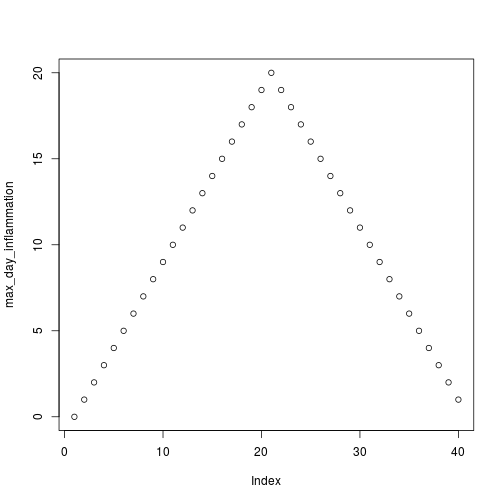
max_day_inflammation <- apply(dat, 2, max)
plot(max_day_inflammation)

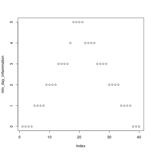
min_day_inflammation <- apply(dat, 2, min)
plot(min_day_inflammation)

The maximum value rises and falls perfectly smoothly, while the minimum seems to be a step function. Neither result seems particularly likely, so either there’s a mistake in our calculations or something is wrong with our data.

Answers to challenge exercises: starting-with-data-answers.R